Vuze 3D Stitcher
Create a 3D 360 VR image from 8 fisheye images.
Project maintained by e-regular-games Hosted on GitHub Pages — Theme by mattgraham
World Seams
Date: March 5th, 2023
Script: vuze_merge.py
Usage:
rm -f coeffs_v6.json
src/vuze_merge.py -a coeffs_v6.json --setup camera_setup.json
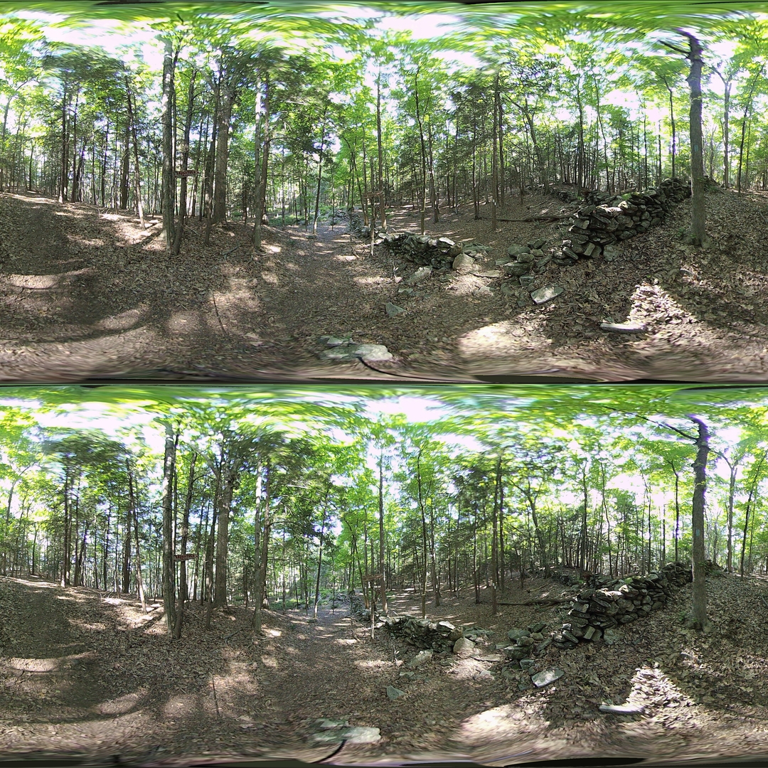
src/vuze_merge.py -a coeffs_v6.json -I test/HET_0014 -O test/HET_0014_world_seams \
--write-coeffs --ignore-alignment-seams
src/vuze_merge.py -a coeffs_v6.json -I test/HET_0017 -O test/HET_0017_world_seams
convert test/HET_0014_world_seams.JPG -resize 25% test/HET_0014_world_seams.JPG
convert test/HET_0017_world_seams.JPG -resize 25% test/HET_0017_world_seams.JPG
Objective
Refine the fisheye to 3D 360 panorama stitching process to account for depth and to intelligently choose seams based on depth, seam quality, and position. The current process for converting the fisheye images to a single 3D 360 panorama relies on averaging the location of feature points between the left and right side for a single eye. The idea will be to determine the depth of various feature points and use the detph along with known characteristics of the human head to convert to a 3D 360 image which when viewed by a person accurately represents the world from the individual lens images. First, a coordinates system for each space needs to be defined.
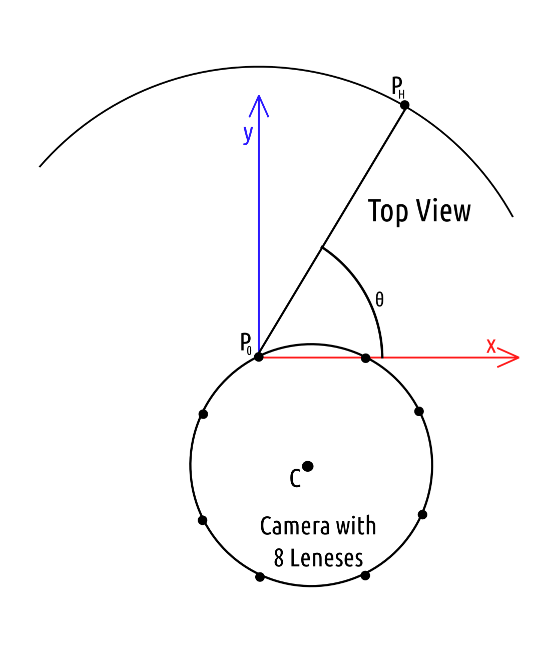
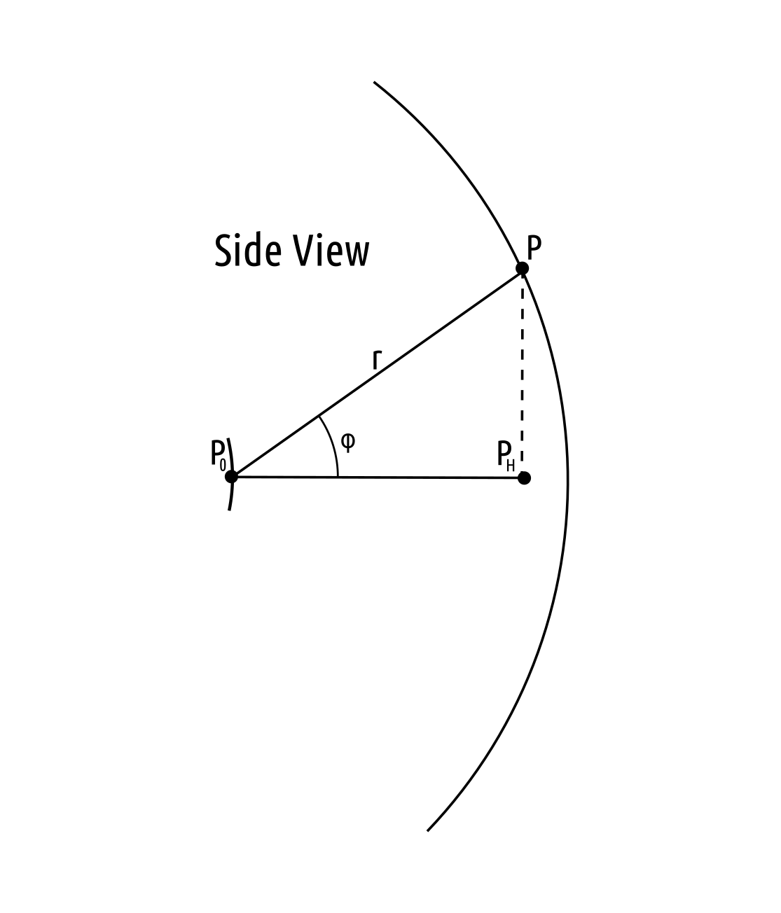
Lens Coordinates
Each lens takes a single fisheye image centered around its position on the camera. Each pixel in the images is represented as $(\phi, \theta)$ pair centered at the lens origin, cartesian point $P_0$. The polar coordinates can be convereted to a cartesian coordinates using the estimated radius for that location, $r$. The cartesian point will be $P$.
| Top View | Side View |
|---|---|
 |
 |
Eye Coordinates
The eye coordinate system will be used to identify locations within the final $360^{\circ}$ polar image. These polar coordinates can easily be converted to equirectangular coordinates in order to generate the final image. The coordinate system must be able to adjust to each eye and be consistent across all sides of the camera and all vertical view rotations.
| Top View | Side View |
|---|---|
 |
 |
Determining the Radius
For simplicity the radius was chosen to be 5m in all case. The radius can be computed using the depth calculations from Depth Calibration. Using this process with determined feature points many issues arose regarding the quality of the alignment of the images. The radius along the seam turned out to be inaccurate and thus a fixed 5m was used.
The investigation into determining the radius used feature points from all 4 overlapping lens images to create a depth map. The depth map was based on the cloud of determined feature points and their radius calculated using the respective position of each lens. The depth map used the N nearest points to a provided point and took a weighted average by distance to determine an estimate for the radius.
Lens to Eye Transform
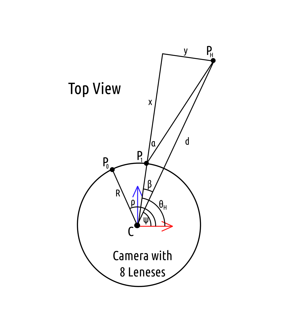
The forward transformation will be applied in 2 steps; first calculate $\theta_H$, then calculate $\phi_H$. The input and output coordinates of the transform will be polar with the left side of the image at $\frac{\pi}{2}$ radians and the right side of the image at $\frac{3\pi}{2}$ radians. This is oposite and offset from the lens coordinates system defined above. For simplicity the plane of the camera is assumed to be the x-y-axis plane, ie. $z=0$. The objective is to find $(\phi_H, \theta_H)$. A required input is the interocular distance, $E$, in meters.
\[P_H = \vec{P_0} + \begin{pmatrix} r \sin \left( \phi \right) \cos \left( \frac{3\pi}{2} - \theta \right) \\ r \sin \left( \phi \right) \sin \left( \frac{3\pi}{2} - \theta \right) \\ 0 \end{pmatrix}\] \[\begin{array} & R = \left\| \vec{p_0} \right\| & \alpha = \sin^{-1} \left( \frac{E}{2R} \right) & y = x \tan(\alpha) & d = \left\| P_H - C \right\| \end{array}\] \[\begin{align} d^2 &= ( R + x )^2 + y^2 \\ d^2 &= ( R + x )^2 + x^2 \tan^2(\alpha) \\ d^2 &= x^2 + 2Rx + R^2 + x^2 \tan^2(\alpha) \\ 0 &= \left( 1 + \tan^2(\alpha) \right) x^2 + 2Rx + (R^2 - d^2) \end{align}\]This yields an equation with two solutions for $x$. The quadratic formula is used and the solution which will yield a positive $x$ in all cases is selected.
\[\begin{align} x &= \frac{-2R + \sqrt{4R^2 - 4 \left( 1 + \tan^2(\alpha) \right) (R^2 - d^2)}}{2 \left( 1 + \tan^2(\alpha) \right)} \\ x &= \frac{-R + \sqrt{R^2 - \left( 1 + \tan^2(\alpha) \right) (R^2 - d^2)}}{\left( 1 + \tan^2(\alpha) \right)} \end{align}\]Using $x$ the angle $\beta$ can be determined.
\[\beta = \cos^{-1} \left( \frac{x + R}{d} \right)\]The final angle $\theta_H$ will be zeroed relative to $\rho$.
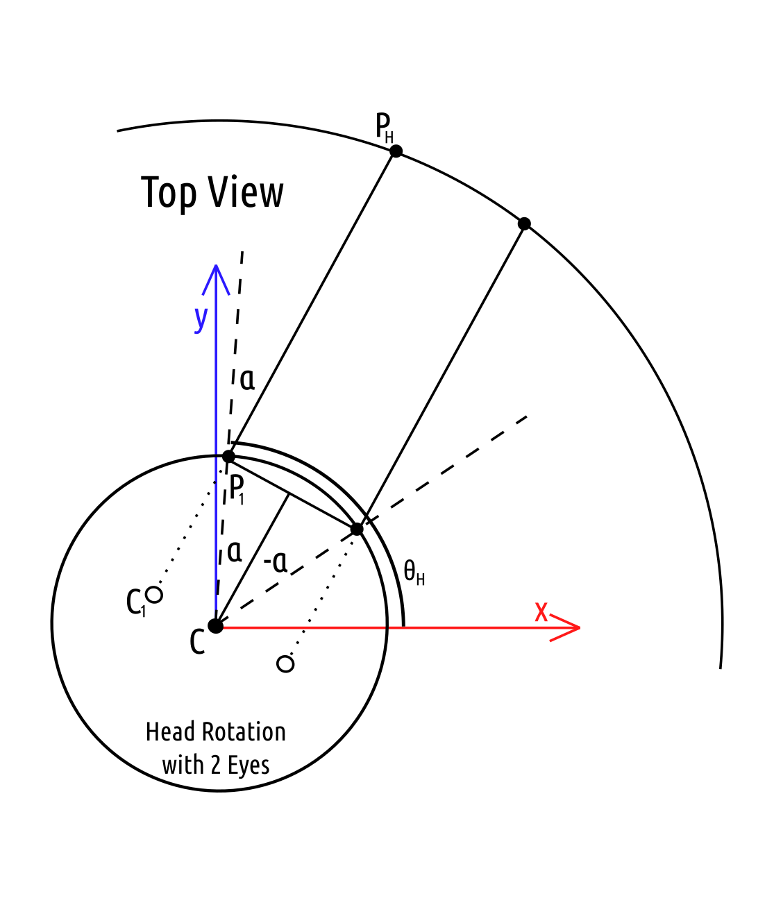
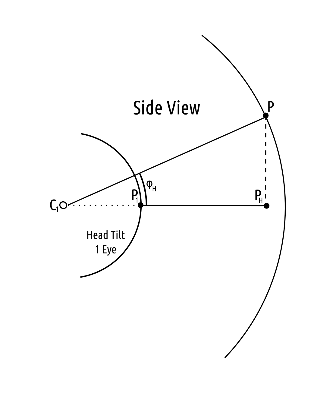
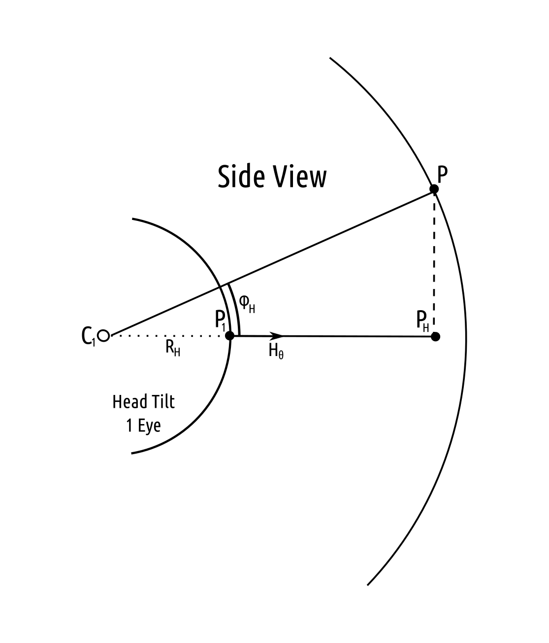
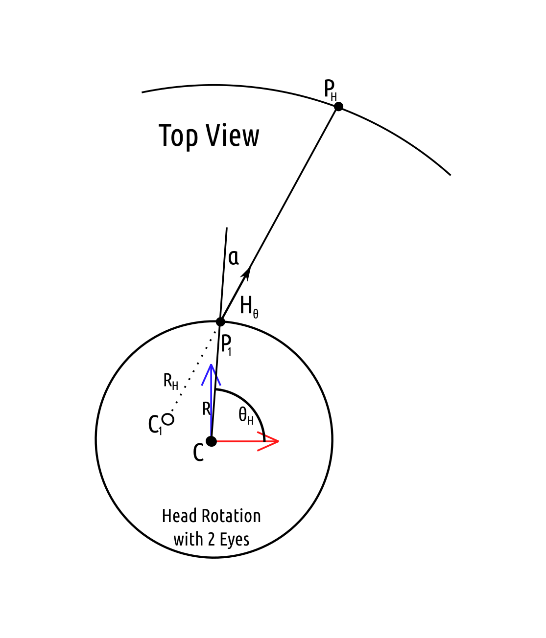
\[\theta_H = \rho - (\beta + \psi)\]The location of $P_1$ and $C_1$ are computed in order to calculate $\phi_H$. The distance $R_H$ is the distance from the eye to the tilt axis of the head behind the eye. The value of $e$ is dependent upon the eye being calculated: $e=1$ for the left eye and $e=-1$ for the left eye.
\[\begin{array} & P_1 = C + \begin{pmatrix} R \cos \left( \psi + e \beta \right) \\ R \sin \left( \psi + e \beta \right) \\ 0 \end{pmatrix} & \vec{H_\theta} = \frac{P_H - P_1}{ \left\| P_H - P_1 \right\| } & C_1 = P_1 - R_H \vec{H_\theta} \end{array}\] \[\phi_H = \cos^{_1} \left( \frac{R_H + \left\| P_H - P_1 \right\|}{ \left\|P - C_1 \right\| } \right)\]The following diagrams labels the distances in a specific example using a location of $P_1$ to the right of $P_0$. The polar coordinate $(\phi_H, \theta_H)$ will need to be converted into the proper orientation with $\phi_H = 0$ being the top of the image and $\theta_H = \pi$ being at the center of the image with $\theta_H = \frac{\pi}{2}$ on the left side.
| Top View | Side View |
|---|---|
 |
 |
Eye to Lens Transform
The transform from eye to lens is a bit more complicated because the distance from the eye to the point is assumed to be unknown. The input and output coordinates of the transform will be polar with the left side of the image at $\frac{\pi}{2}$ radians and the right side of the image at $\frac{3\pi}{2}$ radians. This is oposite and offset from the lens coordinates system defined above. For simplicity the plane of the camera is assumed to be the x-y-axis plane, ie. $z=0$. The objective is to find $(\phi, \theta)$. A required input is the interocular distance, $E$, in meters.
The calculation will be performend using vectors only and trigonometric functions will be avoided. The distance $R_H$ is the distance from the eye to the tilt axis of the head behind the eye. The value of $e$ is dependent upon the eye being calculated: $e=1$ for the left eye and $e=-1$ for the left eye.
\[\begin{array} & R = \left\| \vec{p_0} \right\| & \alpha = -e \sin^{-1} \left( \frac{E}{2R} \right) \end{array}\]Three rotation matrices will be required $R_\alpha$, $R_{\phi_H}$, and $R_z$. The rotation $R_\alpha$ rotates a vector about the x-axis by an angle of $\alpha$. The rotation $R_{\phi_H}$ rotates a vector about the y-axis by an angle of $\phi_H$. The rotation $R_z$ rotates a vector $90^\circ$ about the z-axis.
\[\begin{array} & R_\alpha = \begin{bmatrix} \cos(\alpha) & -\sin(\alpha) & 0 \\ \sin(\alpha) & \cos(\alpha) & 0 \\ 0 & 0 & 1 \end{bmatrix} & R_{\phi_H} = \begin{bmatrix} \cos(\phi_H) & 0 & \sin(\phi_H) \\ 0 & 1 & 0 \\ -\sin(\phi_H) & 0 & \cos(\phi_H) \end{bmatrix} & R_z = \begin{bmatrix} 0 & -1 & 0 \\ 1 & 0 & 0 \\ 0 & 0 & 1 \end{bmatrix} \end{array}\] \[P_1 = \begin{pmatrix} R \cos(\theta_H) \\ R \sin(\theta_H) \\ 0 \end{pmatrix}\] \[\vec{H_\theta} = \frac{R_\alpha P_1}{ \left\| P_1 \right\| }\]The objective is to determine the vector from $C_1$ in the direction $\vec{H_\phi}$ of $P$. The exact value of $P$ will be the final result and using it the polar coordinates of $P$ from $P_0$ can be computed. Once the vector from $C_1$ is determined its intersection with the sphere centered at $P_0$ with radius $r$ will be determined.
\[C_1 = P_1 - R_H \vec{H_\theta}\]To determine $H_\phi$ the vector $H_\theta$ will be rotated about $C_1$ by the angle $\phi_H$. This will require create a basis for the space which allows for easier rotation using $R_{\phi_H}$. Since $\vec{H_\theta}$ is in the x-y-axis plane the $R_z$ rotation can be used to create a perpendicular unit vector. The basis will be defined as follows. Using this bases the unit vector in the x-direction can be rotated by $R_\phi$ and then untransformed from this bases to obtain $\vec{H_\phi}$.
\[T_H = \begin{bmatrix} & \vec{H_\theta} & \\ & R_z \vec{H_\theta} & \\ 0 & 0 & 1 \end{bmatrix}\] \[\vec{H_\phi} = T^T_H R_\phi \begin{pmatrix} 1 \\ 0 \\ 0 \end{pmatrix}\]Now the intersection $P$ can be computed.
\[P = C_1 + d \vec{H_\phi}\] \[\left\| P - P_0 \right\|^2 = r^2\]Using the intersection of a line and sphere from Wikipedia there are two possible solutions for $d$. Again the solution which yields a positive value for $d$ is used. The radius from $P_0$ to $P$ was assumed to be a constant value for all points.
\[d = -\vec{H_\phi} \cdot (C_1 - P_0) + \sqrt{ \left( \vec{H_\phi} \cdot (C_1 - P_0) \right) ^2 - \left( \left\| C_1 - P_0 \right\| ^2 - r^2 \right)}\]This $d$ can be used to compute $P$ and the polar coordinates of $P$ from $P_0$ yield $(\phi, \theta)$.
| Top View | Side View |
|---|---|
 |
 |
Intelligent Seam Determination
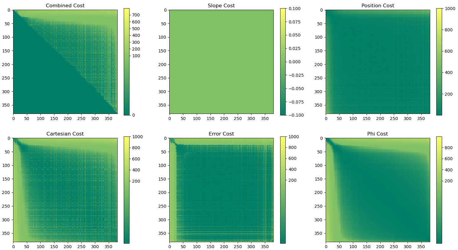
To determine the best path along a seam the matching feature points from each lens will be used as possible points along the path. The cost to move between points is calculated as the weighted average of 5 metrics. These metrics are based on the polar path between the nodes along the arc determined by a linear progression of $\phi$ and $\theta$. The arc is divided into 50 discrete segments which are used to estimate the values along the path.
The Error, $C_e$, cost between nodes is the error from the linear regression used to ensure the feature points from each image align in the final head coordinate space.
The Cartesian, $C_c$, cost is the distance measured between the cartesian coordinates along the image sphere. This measure accounts for the radius of each point along the sphere when calculating the coordinates.
The Phi, $C_\phi$, cost is the difference between $\phi$ of different nodes.
The Slope, $C_s$, cost is most relevant when the radius of the sphere is allowed to change with respect to the polar coordinate. It represents the changes in the radius with respect to changes in the polar coordinates. The increased cost with increased slope will deter selections of points in which there are drastic changes in the radius.
The Position, $C_p$, cost is the distance between pairs of polar coordinates $(\phi, \theta)$ by taking the norm of the difference between polar points along the path.
Each cost is squared and scaled such that the minimum value is 1 and the maximum value is 1000. The costs are then combined using the following weights.
\[0.5C_e + 0.2C_s + 0.1C_c + 0.1C_p + 0.1C_\phi\]The path with the lowest cost is determined using the scipy.sparse.csgraph.shortest_path function. An example of the cost used as input to the function is provided below. The HET_0014 images is used to generate the example and the seam lengths for the image are detailed below.
| Cost between Nodes |
|---|
 |
| Seam | Length |
|---|---|
| 1 | 18 |
| 2 | 17 |
| 3 | 18 |
| 4 | 19 |
Results
To verify the transforms were working as expected a matrix of polar coordinates were run through the forward calculations and then the reverse. The intial value with the final values were compared and the difference was seen to be extremely close to 0. A similar process was performed using the reverse and then forward calculation and again the result was extremely close to 0.
| HET_0014 with new Transforms |
|---|
 |
| HET_0017 with new Transforms |
|---|
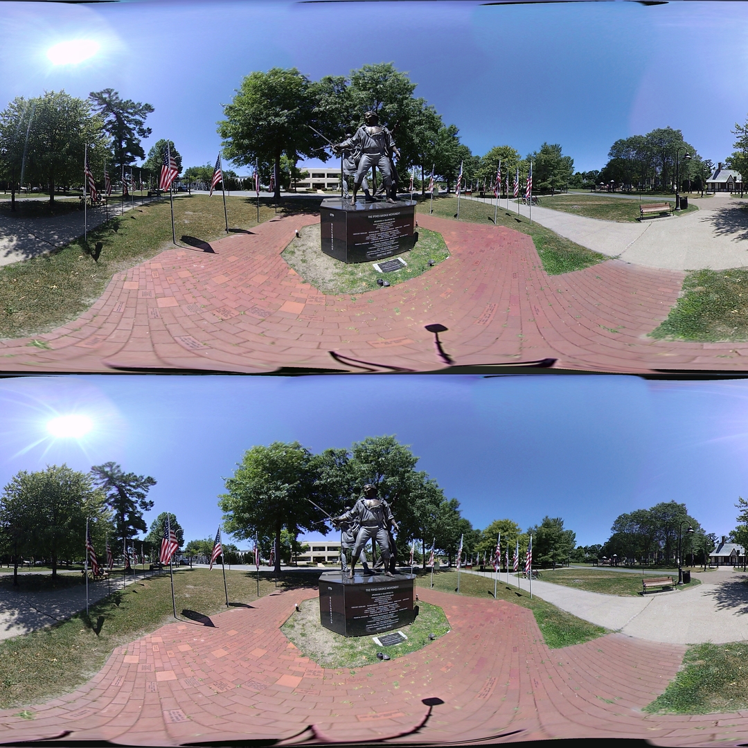 |
Saved Calibration Configuration
The calibration process specification was simplified and directly presented in a single configuration file, example. This reduces the knowledge required to run multiple commands in the proper sequence. The new configuration file is specified in a single command and the script is responsible for executing the calibration steps in the correct order. The provided alignment file will be created or updated.
Source File: camera_setup.py
Usage:
src/vuze_merge.py --alignment coeffs_v6.json --setup camera_setup.json
Questioning Assumptions
Is $\phi$ the same for a given point between 2 lenses?
Short answer: No
The setup uses 2 cameras at $c_1$ and $c_2$ in the same y-plane and z-plane, and 1 point at $P$. Represented in cartesian coordinates as follows.
\[\begin{array}{cc} c_1 = \begin{pmatrix} c_{x1} \\ c_y \\ c_z \end{pmatrix} & c_2 = \begin{pmatrix} c_{x2} \\ c_y \\ c_z \end{pmatrix} & P = \begin{pmatrix} P_x \\ P_y \\ P_z \end{pmatrix} \end{array}\]From each camera the point $P$ appears at the following locations.
\[\begin{array}{cc} P_1 = \begin{pmatrix} P_x - c_{x1} \\ P_y - c_y \\ P_z - c_z \end{pmatrix} & P_2 = \begin{pmatrix} P_x - c_{x2} \\ P_y - c_y \\ P_z - c_z \end{pmatrix} \end{array}\]Next Convert to polar coordinates and specifically calculating $\phi$.
\[\phi_1 = \cos^{-1} \left( \frac{P_z}{ \sqrt{ \left( P_x - c_{x1} \right) ^2 + P_y^2 + P_z^2 } } \right)\] \[\phi_2 = \cos^{-1} \left( \frac{P_z}{ \sqrt{ \left( P_x - c_{x2} \right) ^2 + P_y^2 + P_z^2 } } \right)\]Given the slight difference in the formulas arising from the difference in the $x$ location of the cameras the asumption that the value of $\phi$ between the two cameras should be the same is an incorrect assumption.